Lidar 2D

Overview

A 2D lidar is a sensor that spins a laser and measures the distance to the first obstacle it meets, hundreds of times per revolution. The result is a horizontal slice of the room: a list of distances, one per angular step. Onlyview turns that slice into 3D geometry, removes everything that belongs to the room itself (walls, furniture), groups what is left into blobs, and tracks those blobs over time — which gives you the live position of the people walking in front of the sensors, without them wearing anything.

The output is a Trackings value, the same type produced by TUIO Input or consumed by the Followspot nodes, so it can drive projections, be re-sent as TUIO to another machine, or move a 3D object.

This device needs more user work than the others: nearly everything happens in the ActionGraph, in a chain of nodes that you have to build and tune yourself. Covering a large room usually means several sensors, so the graph ends up with one branch per sensor, all merged before tracking. Plan for a couple of hours of tuning on site.

Info

Onlyview connects to the sensors from the master only (the Producer in a normal setup). Media Servers do not open any connection to the lidars: the blob tracking is computed on the Producer and the result is sent to them over the show network, so every machine agrees on the same tracked positions.

Hardware

The plugin speaks SICK's binary CoLa B protocol over TCP, on the fixed port 2112, and asks the sensor for a continuous LMDscandata stream. It has been tested with the SICK TiM series.

What Onlyview reads from each scan:

• The DIST1 channel only — the distance of the first echo, converted to metres. Second echoes and the RSSI (energy) channels are skipped.
• The angular span of the scan (angle step × number of samples), which it uses to spread the rays around the sensor's axis.

Onlyview never configures the sensor: the angular range, the resolution and the scan frequency are whatever the sensor itself is set to, and the number of rays you get in the ActionGraph follows from that.

Before creating the device in Onlyview:

• Give each sensor a fixed IP address, with SICK's SOPAS tool, and check that the Producer can reach it (using ping).
• Mount the sensor level, so that its scan plane is horizontal, at the height where you want the slice to be taken. Around ankle height is the usual choice for tracking people.
• Keep the sensors away from mirrors, glass and glossy floors.

Setup

The setup dialog has two fields:

• Device name: free text; it is what you see in the node's Device property and on the UserScreen widget.
• IP Address: the sensor's address. The port is not configurable.

Create one device per sensor. Onlyview connects when the show is loaded and, if the connection fails or drops, retries every 5 seconds, indefinitely — so a sensor that is powered up late, or rebooted during the show, comes back on its own.

Device Widget

Dropped on a UserScreen, the device shows its name (prefixed with [LIDAR]) and one status square. The square is green only when the TCP connection is up and a scan has been received in the last second; anything else — sensor unplugged, sensor connected but not streaming — turns it red. With one widget per sensor, this is the quickest way to check a whole rig before a show.

Placing the sensors in the 3D scene

The device only reports distances; it knows nothing about where it is. You need to tell Onlyview where each sensor stands, and this is what makes the measurements land in the right place in your 3D scene.

The usual method is one empty Object3D per sensor, positioned and rotated to match the physical installation, and read back with a Get Object 3D Transform node (in World space) wired to the Lidar2D Device node's Device position and Device rotation inputs. Editing a transform in the 3D scene, with the room geometry visible around it, is far more practical than typing coordinates into the node.

How the rays are laid out around that transform:

• They all start at the object's origin.
• They stay in the object's local XZ plane — horizontal, if the object is not tilted.
• The fan is centred on the object's local +X axis, and spans the angular range reported by the sensor (so ±135° for a 270° sensor)

So: point the empty's +X axis at the middle of the sensor's field of view, and in practice only the Y rotation (yaw) needs to be adjusted.

Warning

Give every sensor of the same rig the same height — its real mounting height. Blob clustering happens in 3D: if two sensors are entered 20 cm apart vertically while Max points distance is 10 cm, the points they measure on the same person can never end up in the same blob, and one visitor is tracked as two.

Two habits that make the on-site alignment much easier:

• Parent all the empties to a single object. The whole rig can then be shifted and rotated at once, which is what you need when the 3D model of the room and the room itself disagree by a few centimetres.
• Draw the rays while you align (see Debugging). A correctly placed sensor produces rays that stop exactly on the walls of the 3D model. Aligning on the walls is easy, precise, and it validates the position, the rotation and the scale of your scene in one go.

The pipeline

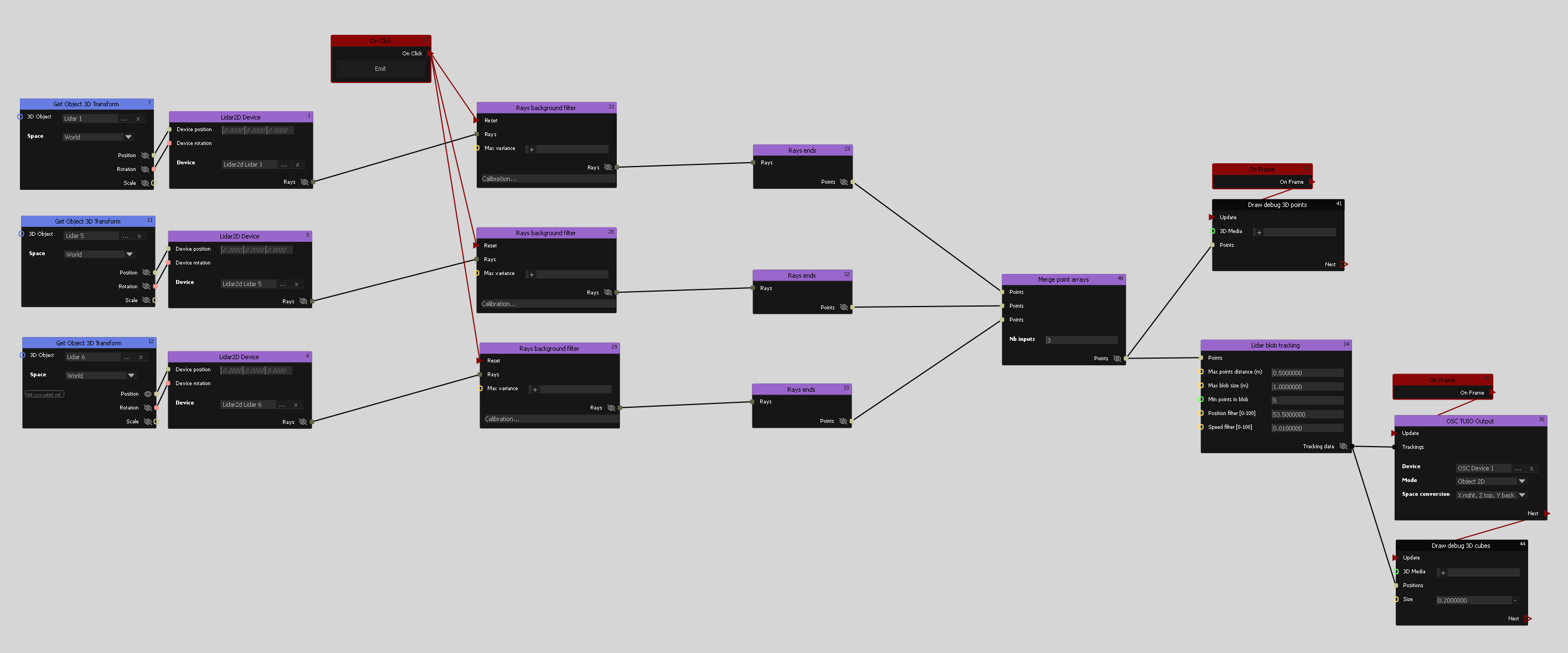
From left to right, per sensor: the transform of the empty feeds a Lidar2D Device node, which outputs raw rays; a Rays background filter keeps only the rays that hit something that is not part of the room; Rays ends turns those rays into a list of points. All the branches then join into one Merge point arrays, whose point cloud goes into Lidar blob tracking, and the resulting Trackings value is sent out — here with an OSC TUIO Output node.

Note the On Click node wired to the Reset event of every background filter: that is how you re-run the background calibration by hand, from the graph. For a show, replace it with an On Action node so a QuickKey or a Command Cue can do it, or with a UserScreen push-button.

All these nodes live under Devices/Lidar2D in the node palette.

Lidar2D Device

Outputs the current scan as rays in world space.

Properties

• Device: the Lidar2D device to read from.

Inputs

• Device position (Vec3): where the sensor stands, in world space.
• Device rotation (Quat): how it is oriented — see Placing the sensors.

Outputs

• Rays (Rays3D): one ray per angular step of the scan, each going from the device position to the point where the beam hit something.

Rays background filter

This is the node that separates the room from what moves in it, and the one that needs the most care.

It starts by learning a background: for each ray index it averages the measured distance over about 200 evaluations — roughly 8 seconds at 25 fps — and at the same time computes how much that distance fluctuates. A label at the bottom of the node shows Calibration... while this is running, then Calibrated. No point comes out of the node during calibration.

Warning

The room must be empty while a filter calibrates, otherwise whoever is standing there becomes part of the background and stops being detected. On a show that runs unattended, keep in mind that calibration restarts when the show is loaded.

Once calibrated, a ray is kept only if all of the following hold:

• Its distance is at least 20 cm shorter than the background. Something has come between the sensor and the wall.
• Its distance is more than 10 cm from the sensor. Closer than that is treated as garbage.
• Its measured distance during calibration was stable enough — see Max variance below.

A ray that reads longer than the background is dropped rather than trusted: the usual explanation is a slightly reflective surface that the sensor stopped seeing directly, not an obstacle.

The node then cleans up the edges of each group of consecutive kept rays. The first and last ray of a group are the ones that just skim past a person, and they tend to flicker between the person's distance and the wall behind; each is discarded if it reads more than 50 cm further than its inner neighbour. Groups of a single ray are discarded as noise.

Inputs

• Rays (Rays3D): from the Lidar2D Device node.
• Max variance: the largest fluctuation, measured during calibration, that a ray may have and still be usable. Leave the field empty to disable the test (the default): every ray is then usable regardless of how noisy it was. Set a value to get rid of rays that never settle — those grazing an edge, or aimed at a curtain, a plant, or anything else that moves slightly but permanently. The value is a variance, in m², so it grows quadratically: tighten it gradually until the false detections disappear.

Events

• Reset: throws the background away and calibrates again. Use it after moving scenery, or whenever detection has become visibly wrong.

Outputs

• Rays (Rays3D): the rays that were kept, unchanged.

One filter is needed per sensor: the background is a list of distances per ray index, so it only makes sense for one sensor's stream.

Info

The background is learned once and never updated afterwards. This is deliberate — a slowly adapting background would swallow anyone standing still — but it means that a chair moved during the day stays a "hole" in the background until the next Reset. Make the reset reachable during the show (QuickKey, UserScreen button) rather than only in the graph.

Rays ends

Converts rays into points, by keeping the target of each ray: the spot where the beam hit something.

Inputs: Rays (Rays3D). Outputs: Points (Vec3s).

The node is only there to make the pipeline explicit. Onlyview converts Rays3D to Vec3s automatically, exactly the same way, so you can also connect a Rays output straight into a Points input and skip the node entirely.

Merge point arrays

Concatenates several point lists into one, so a single blob tracker sees all the sensors at once.

Properties

• Nb inputs: how many Points inputs the node has; the node's slots update as soon as you change it.

Inputs: Points (Vec3s) × Nb inputs. Inputs that carry no valid value are simply skipped, so a disconnected sensor does not break the others.

Outputs: Points (Vec3s) — all the input points, one after the other. The output is invalid when the total is empty.

Merging before tracking, rather than tracking each sensor separately, is what makes a visitor seen by two sensors a single tracked person, and what lets one sensor take over when another is occluded.

Make a point array is the same idea for individual points: it takes Nb inputs Vec3 values and bundles them into a Vec3s. Handy to inject a hand-placed point into the pipeline while testing.

Lidar blob tracking

Groups the point cloud into blobs, and follows those blobs from frame to frame.

Inputs

• Points (Vec3s): the merged point cloud.
• Max points distance (m) — default 0.1: how far apart two points may be and still belong to the same blob. Too small and one person breaks into several blobs; too large and two people standing close merge into one. This is also what has to bridge the gap between the arcs measured by two different sensors on the same person.
• Max blob size (m) — default 0.5: the largest radius a blob may reach. Points further than this from the blob's centre are not added to it, which stops a blob from growing along a wall or swallowing a queue of people.
• Min points in blob — default 2: blobs made of fewer points are ignored. Raise it to reject noise; a person far from the sensor only returns a few points, so raising it too much creates a maximum detection distance.
• Position filter [0-100] — default 20: how strongly a new measurement pulls the tracked position (the α of an alpha-beta filter). 100 means "jump straight to the measurement", low values mean heavy smoothing and a visible lag. Do not set it to 0, the position would never move.
• Speed filter [0-100] — default 10: how strongly a new measurement updates the estimated velocity (the β of the same filter). The velocity is what extrapolates a blob's position while it is momentarily hidden, and it is also reported in the output; a low value makes it almost inert, which is often what you want with slow-moving visitors.

Outputs

• Tracking data (Trackings): one entry per tracked blob, with an id, a filtered position, an estimated velocity, and the timestamps of its first and last sighting.

How the tracking behaves, in practice:

• Existing blobs get first pick. Each frame, every known blob is extrapolated with its velocity and looks for points around that predicted position; only the points nobody claimed can form new blobs. This is what keeps ids attached to the same person when two people walk past each other.
• A blob survives 500 ms unseen. While it is missing, its position keeps moving along its last known velocity, and it disappears if it has not been seen again after half a second. Brief occlusions therefore do not break a track.
• A new blob is published after 500 ms. A freshly created blob is held back from the output until it is half a second old, which filters out the flicker of a bad reflection — at the price of half a second of delay before a visitor entering the room is reported.
• Ids are never reused. They increase for the lifetime of the show. A person lost for more than 500 ms comes back as a new id, so do not use the id as a durable identity.
• No orientation. A blob is a group of points with no shape and no facing direction; the rotation carried by the Trackings value is not meaningful.

This node runs on the master only, and broadcasts its result to the Media Servers, so every machine tracks identically. Its inputs are read on the master too: changing them affects the whole show.

Lidar2D Simulator

Replaces a real sensor with a synthetic one, so a pipeline can be built and tested with no hardware at all. It outputs Rays exactly like the Lidar2D Device node, and plugs into a background filter in the same way.

Inputs

• Device position (Vec3) and Device rotation (Quat): as on the real node.
• Beam angle (°) — default 180: angular span of the simulated fan.
• Rays count — default 100: number of rays in it.
• Timecode: the time, in milliseconds, that drives the animation. Connect Show Clock (ms) (see Miscellaneous).

What it simulates is fixed and cannot be configured: a rectangular room roughly 9 × 5.5 m centred on the origin, and two 50 cm wide, 1.7 m tall cylinders — the "people" — wandering inside it on their own trajectories. A little noise is added to both the distances and the ray angles, on purpose: real sensors do that, and it makes background filtering realistically hard.

So place the simulated sensor inside that room — somewhere within x ∈ [−5, 4], z ∈ [−3, 2.5], at a height between 0 and 1.7 m — otherwise it sees nothing but walls, or nothing at all. It is a test bench for the graph, not a preview of your venue.

Debugging

Nothing in the pipeline is visible by itself, so the Debug Draw nodes are the only way to see what is going on. The same graph as above, with drawers added at each stage:

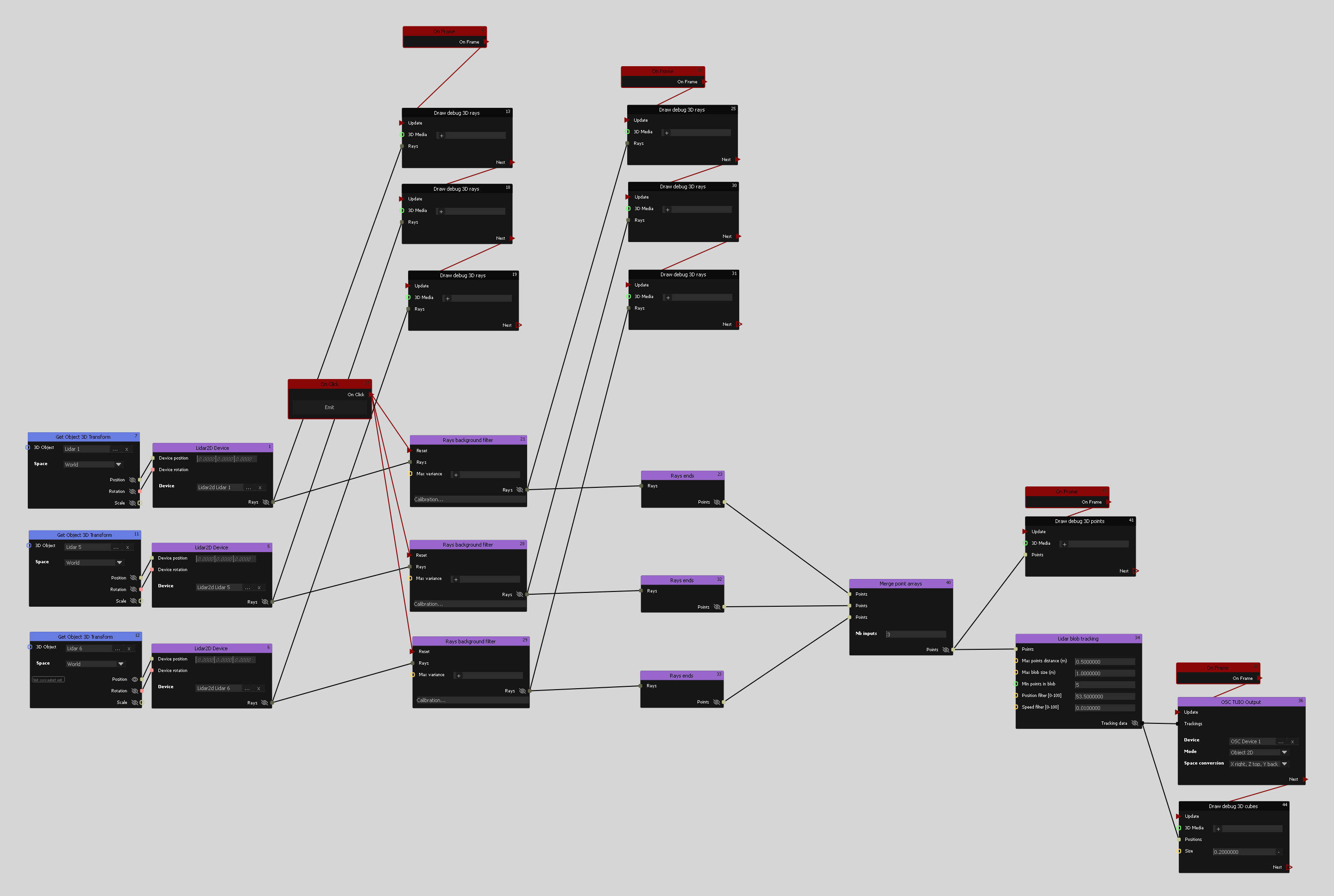
• Draw debug 3D rays on a Lidar2D Device output shows the raw scan. This is the view to use for aligning the sensors: the rays must stop on the walls of the 3D model.
• Draw debug 3D rays on a background filter output shows what survived the filtering — ideally only the rays that hit people. Stray rays pointing at a wall mean the background needs a Reset, or that Max variance should be tightened.
• Draw debug 3D points on the merged cloud shows the point cloud the tracker actually receives, all sensors together.
• Draw debug 3D cubes on the tracking positions shows the tracked people. Set Size to something person-sized (0.2 m in the picture) and watch whether the cubes stay put, jitter, split in two or swap places.

Each drawer needs its Update event driven by an On Frame event, and its 3D Media input set to the 3D media you are looking at. Remember that the raw rays and points only exist on the master: the ray and point overlays show up in the Producer's 3D preview, while the tracking cubes, which come from synchronised data, appear everywhere.

Using the tracking data

The Trackings value coming out of the blob tracker is a standard Onlyview type, and the lidar pipeline is just one possible source for it:

• OSC TUIO Output re-sends it as TUIO to another machine — TouchDesigner, Unreal, a web page… Pick the Mode and Space conversion that the receiving software expects.
• The Followspot nodes aim real fixtures at tracked people.
• Any node taking a Trackings input works the same way, whether the data comes from a lidar rig, from TUIO Input, or from a camera-based system.

Limitations

• One horizontal slice, and nothing else. There is no height information, no shape, no orientation, and no way to tell a person from an object of the same size. Anything hidden behind something else at sensor height is invisible — which is the reason for using several sensors and merging their clouds.
• The background is learned once, in an empty room, and only re-learned on a Reset.
• No sensor configuration from Onlyview. Range, resolution and scan frequency are set in the sensor itself with SOPAS ET; the TCP port is fixed at 2112 and the sensor's own start angle is ignored.
• Ids are not a durable identity: they change after an occlusion longer than half a second, and a visitor is only reported half a second after entering.
• Only the first echo (DIST1) of each measurement is used; multi-echo and reflectivity data, which could help with glass and reflective floors, are not read.